ClickHouse/docs/en/getting-started/example-datasets/environmental-sensors.md

slug	sidebar_label
/en/getting-started/example-datasets/environmental-sensors	Environmental Sensors Data

Environmental Sensors Data

Sensor.Community is a contributors-driven global sensor network that creates Open Environmental Data. The data is collected from sensors all over the globe. Anyone can purchase a sensor and place it wherever they like. The APIs to download the data is in GitHub and the data is freely available under the Database Contents License (DbCL).

:::important The dataset has over 20 billion records, so be careful just copying-and-pasting the commands below unless your resources can handle that type of volume. The commands below were executed on a Production instance of ClickHouse Cloud. :::

1. The data is in S3, so we can use the s3 table function to create a table from the files. We can also query the data in place. Let's look at a few rows before attempting to insert it into ClickHouse:

SELECT *
FROM s3(
    'https://clickhouse-public-datasets.s3.eu-central-1.amazonaws.com/sensors/monthly/2019-06_bmp180.csv.zst',
    'CSVWithNames'
   )
LIMIT 10
SETTINGS format_csv_delimiter = ';';

The data is in CSV files but uses a semi-colon for the delimiter. The rows look like:

┌─sensor_id─┬─sensor_type─┬─location─┬────lat─┬────lon─┬─timestamp───────────┬──pressure─┬─altitude─┬─pressure_sealevel─┬─temperature─┐
│      9119 │ BMP180      │     4594 │ 50.994 │  7.126 │ 2019-06-01T00:00:00 │    101471 │ ᴺᵁᴸᴸ     │ ᴺᵁᴸᴸ              │        19.9 │
│     21210 │ BMP180      │    10762 │ 42.206 │ 25.326 │ 2019-06-01T00:00:00 │     99525 │ ᴺᵁᴸᴸ     │ ᴺᵁᴸᴸ              │        19.3 │
│     19660 │ BMP180      │     9978 │ 52.434 │ 17.056 │ 2019-06-01T00:00:04 │    101570 │ ᴺᵁᴸᴸ     │ ᴺᵁᴸᴸ              │        15.3 │
│     12126 │ BMP180      │     6126 │ 57.908 │  16.49 │ 2019-06-01T00:00:05 │ 101802.56 │ ᴺᵁᴸᴸ     │ ᴺᵁᴸᴸ              │        8.07 │
│     15845 │ BMP180      │     8022 │ 52.498 │ 13.466 │ 2019-06-01T00:00:05 │    101878 │ ᴺᵁᴸᴸ     │ ᴺᵁᴸᴸ              │          23 │
│     16415 │ BMP180      │     8316 │ 49.312 │  6.744 │ 2019-06-01T00:00:06 │    100176 │ ᴺᵁᴸᴸ     │ ᴺᵁᴸᴸ              │        14.7 │
│      7389 │ BMP180      │     3735 │ 50.136 │ 11.062 │ 2019-06-01T00:00:06 │     98905 │ ᴺᵁᴸᴸ     │ ᴺᵁᴸᴸ              │        12.1 │
│     13199 │ BMP180      │     6664 │ 52.514 │  13.44 │ 2019-06-01T00:00:07 │ 101855.54 │ ᴺᵁᴸᴸ     │ ᴺᵁᴸᴸ              │       19.74 │
│     12753 │ BMP180      │     6440 │ 44.616 │  2.032 │ 2019-06-01T00:00:07 │     99475 │ ᴺᵁᴸᴸ     │ ᴺᵁᴸᴸ              │          17 │
│     16956 │ BMP180      │     8594 │ 52.052 │  8.354 │ 2019-06-01T00:00:08 │    101322 │ ᴺᵁᴸᴸ     │ ᴺᵁᴸᴸ              │        17.2 │
└───────────┴─────────────┴──────────┴────────┴────────┴─────────────────────┴───────────┴──────────┴───────────────────┴─────────────┘

2. We will use the following MergeTree table to store the data in ClickHouse:

CREATE TABLE sensors
(
    sensor_id UInt16,
    sensor_type Enum('BME280', 'BMP180', 'BMP280', 'DHT22', 'DS18B20', 'HPM', 'HTU21D', 'PMS1003', 'PMS3003', 'PMS5003', 'PMS6003', 'PMS7003', 'PPD42NS', 'SDS011'),
    location UInt32,
    lat Float32,
    lon Float32,
    timestamp DateTime,
    P1 Float32,
    P2 Float32,
    P0 Float32,
    durP1 Float32,
    ratioP1 Float32,
    durP2 Float32,
    ratioP2 Float32,
    pressure Float32,
    altitude Float32,
    pressure_sealevel Float32,
    temperature Float32,
    humidity Float32,
    date Date MATERIALIZED toDate(timestamp)
)
ENGINE = MergeTree
ORDER BY (timestamp, sensor_id);

3. ClickHouse Cloud services have a cluster named default. We will use the s3Cluster table function, which reads S3 files in parallel from the nodes in your cluster. (If you do not have a cluster, just use the s3 function and remove the cluster name.)

This query will take a while - it's about 1.67T of data uncompressed:

INSERT INTO sensors
    SELECT *
    FROM s3Cluster(
        'default',
        'https://clickhouse-public-datasets.s3.amazonaws.com/sensors/monthly/*.csv.zst',
        'CSVWithNames',
        $$ sensor_id UInt16,
        sensor_type String,
        location UInt32,
        lat Float32,
        lon Float32,
        timestamp DateTime,
        P1 Float32,
        P2 Float32,
        P0 Float32,
        durP1 Float32,
        ratioP1 Float32,
        durP2 Float32,
        ratioP2 Float32,
        pressure Float32,
        altitude Float32,
        pressure_sealevel Float32,
        temperature Float32,
        humidity Float32 $$
    )
SETTINGS
    format_csv_delimiter = ';',
    input_format_allow_errors_ratio = '0.5',
    input_format_allow_errors_num = 10000,
    input_format_parallel_parsing = 0,
    date_time_input_format = 'best_effort',
    max_insert_threads = 32,
    parallel_distributed_insert_select = 1;

Here is the response - showing the number of rows and the speed of processing. It is input at a rate of over 6M rows per second!

0 rows in set. Elapsed: 3419.330 sec. Processed 20.69 billion rows, 1.67 TB (6.05 million rows/s., 488.52 MB/s.)

4. Let's see how much storage disk is needed for the sensors table:

SELECT
    disk_name,
    formatReadableSize(sum(data_compressed_bytes) AS size) AS compressed,
    formatReadableSize(sum(data_uncompressed_bytes) AS usize) AS uncompressed,
    round(usize / size, 2) AS compr_rate,
    sum(rows) AS rows,
    count() AS part_count
FROM system.parts
WHERE (active = 1) AND (table = 'sensors')
GROUP BY
    disk_name
ORDER BY size DESC;

The 1.67T is compressed down to 310 GiB, and there are 20.69 billion rows:

┌─disk_name─┬─compressed─┬─uncompressed─┬─compr_rate─┬────────rows─┬─part_count─┐
│ s3disk    │ 310.21 GiB │ 1.30 TiB     │       4.29 │ 20693971809 │        472 │
└───────────┴────────────┴──────────────┴────────────┴─────────────┴────────────┘

5. Let's analyze the data now that it's in ClickHouse. Notice the quantity of data increases over time as more sensors are deployed:

SELECT
    date,
    count()
FROM sensors
GROUP BY date
ORDER BY date ASC;

We can create a chart in the SQL Console to visualize the results:

6. This query counts the number of overly hot and humid days:

WITH
    toYYYYMMDD(timestamp) AS day
SELECT day, count() FROM sensors
WHERE temperature >= 40 AND temperature <= 50 AND humidity >= 90
GROUP BY day
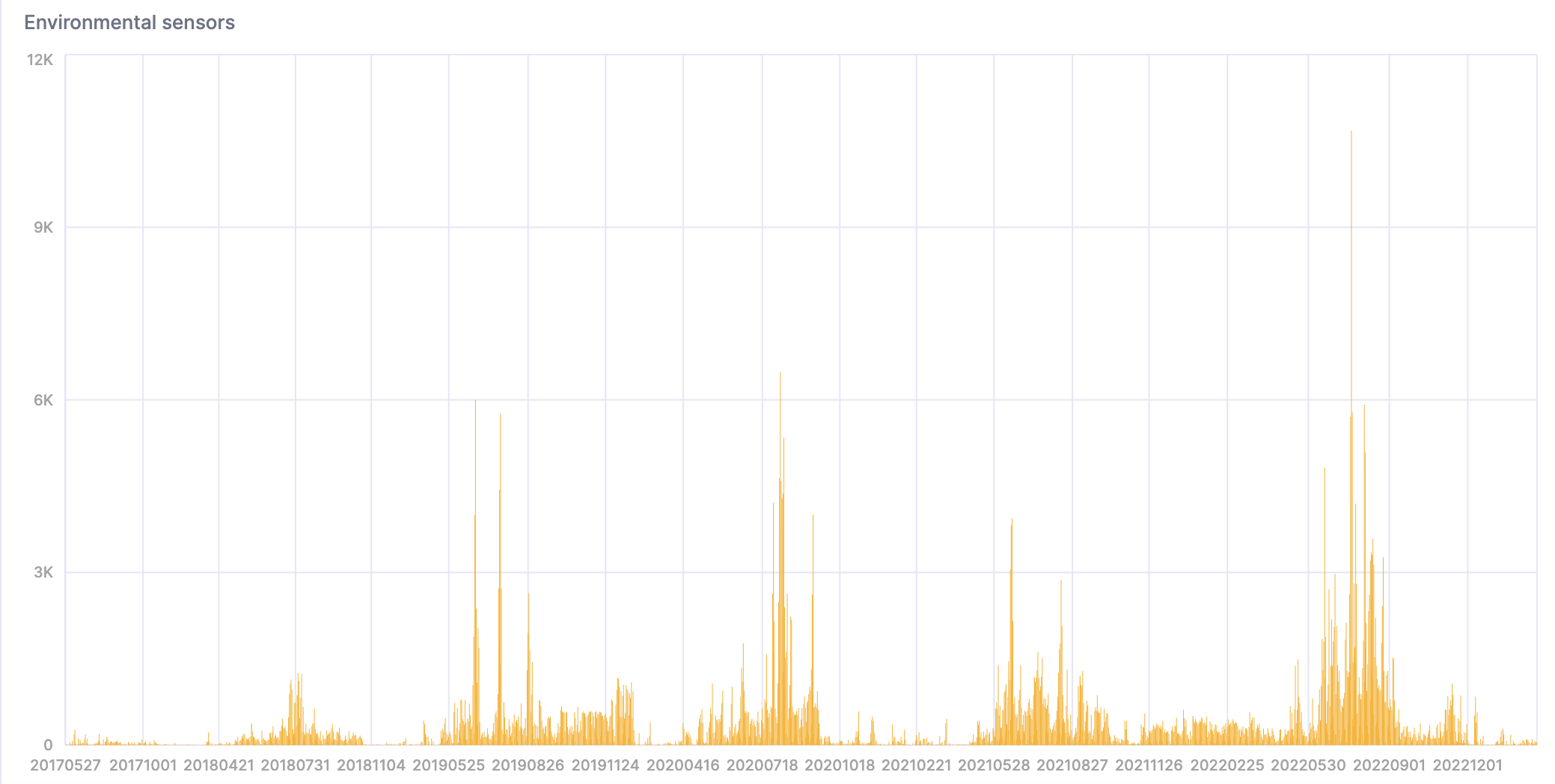
ORDER BY day asc;

Here's a visualization of the result: